Is Aave more conservative than Compound?

[BlockAnalitica]

TLDR

In this post we:

• Show how conservative Aave v3 liquidation thresholds are. We show how it changed over time, and compare it to Compound v3 configurations.
• Compare LTV for different lending pairs as a time-dependent protocol parameter
• Explore different LTV-Borrow Cap pairs and provide tools for active risk management
• Compare Aave v3 to Compound lending markets
• Enhance the huge role that DEX liquidity is playing in the selection of LTV values
• This is done by extending The RiskDAO research for calculating liquidation thresholds and apply to Aave Lending Markets

*This work was a collaboration between Block Analitica and RiskDAO. All authors contributed equally.

Introduction

Deciding on liquidation thresholds comes with few assumptions on how the market will behave in difficult times. These assumptions could include:

• User behavior in a downtrend market.
• Behavior of DEX liquidity in the presence of liquidations.
• Volatility amplification during black swan events
• And more (some of the assumptions have additional sub-assumptions on specific simulation parameters).

In a recent study, the RiskDAO presented a simple formula for calculating liquidation thresholds. This formula takes into account market parameters and a single confidence level factor. This factor aims to represent all the implicit and explicit assumptions with a single number.

In this work, we extend the research and apply it for Aave markets. Our contribution is twofold:

• We extend the methodology and calculate the confidence level factor for Aave markets.
• We compare the confidence level to Compound, and show how these values changed over time (as market conditions have changed).

The outline of this post is as follows. Firstly, we focus on the Price Volatility to be used as input, comparing Parkinson’s volatility estimator with simple Standard Deviation. Next, we concentrate on the confidence level, denoted by c, as a time-dependent parameter, and explore how it can assist us in defining Loan-To-Value (LTV) Ranges of confidence. To benchmark our work, we utilize the WETH-DAI lending pair, which is the most established lending market in DeFi. Finally, we continue our work with a couple of simulations that we believe will be helpful for risk managers in defining LTV and Borrow Cap pairs for any lending protocol. Finally, we compare the c parameter across different Lending Protocols, and enhance the huge role that DEX liquidity is playing in the selection of LTV values.

The confidence level

In their work, RiskDAO proposes a simple formula to determine LTV by means of readily available on-chain data:

where 𝝈 is the annualized price volatility ratio between collateral and debt, β is the liquidation bonus, ℓ and ｄ are the available liquidity and the borrow cap of the debt, respectively, and c is the confidence level factor. It is important to note that for higher values of c the chances of insolvency decrease, and vice versa.

From our perspective, this formula introduces a crucial parameter for risk management to the ecosystem: the confidence level factor, denoted as c. The value of c depends on the risk appetite, but can also depend on qualitative properties of the collateral/debt pair (e.g., centralization risk). Hence, not all lending pairs are equal, necessitating the establishment of a benchmark for c using a well-understood lending pair with underlying assets.

Methodology

The RiskDAO’s formula allows flexibility in the choice of price volatility and whether the focus should be on liquidation events or the time-dependent evolution of returns. Both decisions are challenging. On one hand, using the LTV formula implies that price volatility serves as the primary market indicator for risk management, warranting stress testing in all market conditions.

The choice between focusing on liquidations or the time-dependent volatility over the past years depends on the stage of backtesting and stress-testing of the model. Gathering data to backtest the model can be particularly challenging due to the occurrence of most liquidations during Black Swan Events. Therefore, as an initial approach, we will concentrate on the time-dependent returns and volatility of ETH, WBTC, UNI, DAI, and LINK over the past few years. Additionally, we propose the use of the annualized Parkinson Volatility as an estimation for the price volatility of assets.

This section is divided into four parts. First we will study price volatility for ETH, WBTC, UNI, DAI and LINK, and explore the difference between standard volatility and Parkinson volatility as a risk management tool. In the second part, we will take a look into c and we will construct the boundaries that will determine LTV values for the benchmark lending market ETH-DAI. In part three we perform simulations to show the stark differences between LTV ranges due to factors like Liquidity and Borrow Cap. Finally we take a deep dive into on-chain liquidity data and compare the confidence level factor of different lending markets in Compound and Aave v3.

Price Volatility

It is evident that lower market cap assets like UNI and LINK have different volatility fingerprints than the more established assets ETH and WBTC. This greater volatility is due to different factors like liquidity. The simplest estimator of volatility is the close-to-close realized standard deviation on a rolling window, however, a big chunk of price information is not taken into account. Thinking about risk management, we estimate the price volatility of ETH, WBTC, UNI, DAI and LINK, by means of the Parkinson Volatility over a period of 360 days, using the annualized daily returns, selecting a 14 day rolling subperiod to reduce variance. We further normalize the sample using the collateral-to-debt ratio assuming that the borrower will always acquire debt in DAI when posting collateral. The results are shown by Fig. (1).

Fig. (1). Time-dependent Collateral/Debt Price Volatility for different Lending Pair Markets. UP: Simple close-to-close standard deviation. DOWN: Parkinson Volatility estimator.

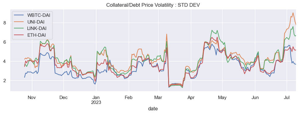
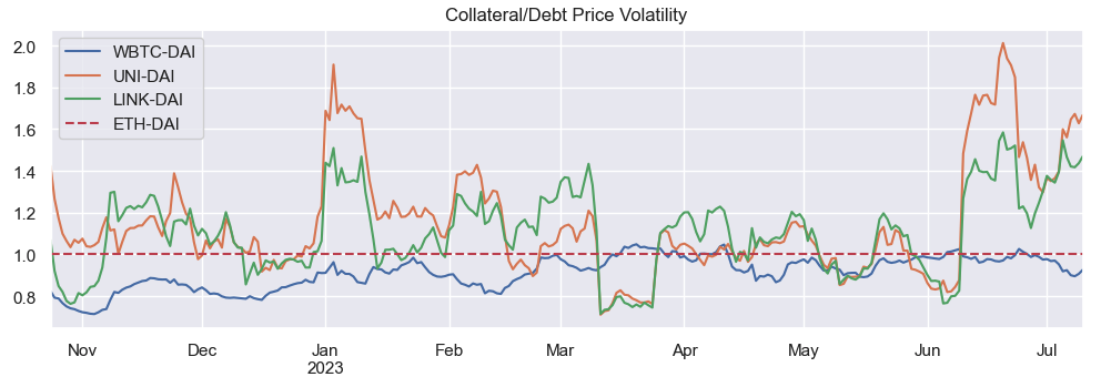
From FIg. (1) it is evident that even though UNI and LINK have clearly more dispersion, by using the Parkinson Volatility we reduce noise in the sample and we standardize the volatility into a tighter range. To simplify the interpretability of the graph above we can benchmark volatility by means of the Price Volatility of WETH-DAI, the most common lending market in DeFi, by simply dividing, as shown in Fig. (2).

Fig. (2). Time-dependent Collateral/Debt Price Volatility for different Lending Pair Markets using the Parkinson Volatility estimator and benchmarking using WETH-DAI.

Confidence Level Factor

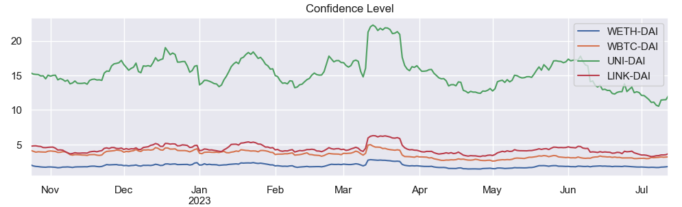
Next, we demonstrate how the ETH-DAI lending market establishes a benchmark for the confidence level by simulatiing its historical behavior on Aave v3 Ethereum market. We accomplish this by utilizing the aforementioned formula and considering time-dependent Price Volatility, as illustrated in Figure (3).

Fig. (3). Time-dependent Confidence Level Factor for different Lending Pair Markets using the Parkinson Volatility estimator and benchmarking using WETH-DAI. For simplicity all data for Borrow Cap, Liquidity and Bonus is constant and was taken from the current Aave v3 Ethereum set parameters. A higher confidence value implies that the LTV configuration is more conservative.

Back to LTV. Finally, considering the time-dependent evolution of the c factor for WETH-DAI, we revisit the formula and establish the LTV ranges based on cmax and cmin. It is crucial to note that the inverse relationship between c and LTV implies that cmax will determine the lowest LTV, and vice versa. This reverse engineering process is shown in Figure (4).

Fig. (4). Time-dependent Loan-To-Value for the ETH-DAI lending market. For simplicity all data for Borrow Cap, Liquidity and Bonus is constant and was taken from the current Aave v3 Ethereum set parameters

LTV - Borrow Cap simulations

Now we focus on a simple simulation to show how different (LTV, Borrow Cap) pairs affect the values of the c factor. For the sake of simplicity we divided price volatility by the benchmark ETH-DAI. Results are shown in Figure (5).

Fig. (5). LTV,BC simulation for the WETH-DAI lending market. For we divided price volatility by the benchmark and kept Bonus constant. In this exercise, we observe how Liquidity affects confidence level factor c.

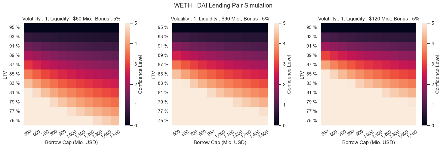
As mentioned by RiskDAO, we show that the LTV formula enables a decision on c instead of LTV. This process entails that, given a confidence level value, a smart contract could autonomously determine the LTV ratio of assets and dynamically adjust it over time. This process will reduce decision-making overhead and facilitate the emergence of an automated and permissionless lending market.

Historical DEX Liquidity

As illustrated in our simulations liquidity plays a huge role when choosing the confidence level factor. Needless to say, liquidity is not constant, therefore we compare on-chain liquidity* over time for some of the most liquid collateral tokens at Aave v3 Ethereum. To calculate asset liquidity we simply get the USD amount that an asset can be sold at a slippage equal to the asset’s liquidation bonus 𝛽. Then we normalize those values with their mean and smooth the results by using a 14 day rolling window.

Fig. (6). Normalized asset liquidity over time for some of the most liquid borrowable assets at Aave v3 Ethereum

Figure (6) exhibits that liquidity can be volatile over time even for these tokens. In the case of ETH we can see that liquidity moved from 60% to 150% of average in the last 18 months.This is even more extreme for WBTC and LINK. These results showcase the complexity of the problem at hand, and highlight the need for dynamical monitoring and revision of LTV values.

Confidence Level across different Lending Protocols

Finally, we compare Aave v3 Ethereum and Compound v3 markets using the LTV formula based on empirical data. Given the current market state, we can quantify the c factor for the same assets across the chosen protocols and for different assets within the same protocol.

Fig. (7). Comparison of computed c factors for chosen assets across Aave v3 Ethereum and Compound v3

The chart above shows that the c-factors are mostly aligned across the two protocols. However, there is a slightly more conservative approach at Aave with LINK and WETH with much more conservative approach with UNI.

Conclusions and Future Work

With this work tackle a multivariate and complex problem using a straightforward quantitative approach. Needless to say, choosing LTV values is a difficult task, but we could conclude that Aave is in general more conservative than Compound. We should also highlight that our research unveils the need for a more dynamic and proactive monitoring and risk management of the protocol, which will help improve user experience and revenue.

[Gauntlet]

We appreciate Block Analitica and RiskDAO’s suggestion. Below we share some feedback to provide the Aave community with further context.

Summary

The methodology provided makes several assumptions around overall market behavior to create an automated mechanism for constructing liquidation thresholds. As a result, it cannot capture important market behaviors that profoundly affect the risk profile of a many-to-many lending platform such as Aave. This can create downstream risk for Aave. So, this amounts to a choice for Aave where the protocol and its community can trade-off between risk and automation. Gauntlet has researched extensively on much of these market behaviors that drive liquidation behavior - below, we will

• Show how these simplifying assumptions and the resulting downstream conclusions can inaccurately conclude that parameters such as liquidation threshold can be loosened without adding excess risk. This may create an inadequate model for the risk profile for Aave.
• Highlight our experience and research around some of the market behaviors assumed in this methodology.

On the Confidence Level Factor

The analysis above seeks to algorithmically compute an asset LT based on a new parameter called the “confidence level factor” c. This confidence factor can depend on the risk appetite and the qualitative properties of the collateral/debt pair. The confidence factor can be increased or decreased based on the community’s preference and perception of the pair.

• This approach may conflate community perception for what an asset’s quality as collateral is, with its actual quality as collateral as characterized by holder distributions, on-chain liquidity, historical and implied volatility, and potential for bad debt.

Validating the correctness of the confidence factor is also challenging. The community will not be able to adapt confidence level factor to changing market conditions, thus potentially leading to stale parameters, despite the LT computation being automatic.

• The underlying aspects of what drive confidence factors can change abruptly. Suppose asset A had a 3 confidence factor. The next day, A drops 20% and liquidity halves 50%. LT automatically adjusts due to the market event, but there is missing feedback for the value of c itself - how does community know that 3 is still the confidence factor to stick with?
• The underlying paper assumes constant liquidity as price decreases, as well as liquidity recovering at constant speed to derive a method to find the confidence factor. We discuss our experience with liquidity in extreme conditions below.

On many to many lending markets

The analysis in the original post is fixated on a [one nonstable collateral - one stable debt] baseline pair to provide some initial insight for the confidence factor. New nonstable collateral - stable debt pairs are then scaled relative to their volatility difference to the baseline. While this framework allows deep analysis into one particular pair, it doesn’t consider the many-to-many nature of Aave v3. The complexities of the relationship between lending parameters and liquidation dynamics explode when multiple assets are introduced.

Suppose a user is supplying $15000 MKR and $15000 SNX and borrowing $18500 USDC, and a price trajectory where at t1 MKR has idiosyncratically dropped 19%, and at t2 MKR has idiosyncratically dropped 28% (SNX has had no change). Consider the two scenarios where scenario 1 is MKR has its current LT (70%), and the second scenario is where we increase the LT of MKR to 80% due to the community’s desire to decrease the confidence factor for MKR / increase LT for MKR. The SNX LT remains the same at 65%. Increasing the LT of MKR implies there is belief that MKR can handle more liquidations during downturns.

scenario	MKR_LT	HF_t1	HF_t2	liquidated_collateral
1	0.7	0.99	1.05	MKR
2	0.8	0.935	0.994	SNX

• In scenario 1, MKR is liquidated at an earlier timestamp, when MKR has only dropped 16%. MKR is chosen to be liquidated due to being more profitable than SNX. Under scenario 2, liquidation is delayed to when MKR has dropped 28%. At this later timestamp, SNX may be liquidated instead because at this timestamp MKR liquidity has significantly dried up. Essentially, increasing the LT for MKR may shift the liquidation volume onto SNX during more extreme price drops.

The liquidation potential of an account is a weighted consideration of all assets supplied and borrowed by the account. The order in which collateral is liquidated and debt is repaid depends on which collateral/debt pair is most profitable. This profitability calculation is a direct output of the slippage and liquidity of the collateral/debt pair. As a result, analyzing risk purely from a single collateral to single debt lens does not capture the second-order effects of LT increases across all assets, which can involve change in liquidation composition at more extreme price drops. This can result in excessively loose parameter recommendations for a many-to-many protocol like Aave.

On some of the assumptions presented in the methodology

Naturally, simple methodologies require simplifying assumptions. When calculating confidence factors, we address some of the assumptions used in the original post.

Constant Slippage

Part of the computation for the confidence factor is rooted in an assumption that slippage of the liquidated collateral asset, as price decreases, remains constant. Above is the pool balance of stETH on Curve, as well as the stETH/ETH price during June 2022. As liquidity declines, the potential for price shocks increase, since similarly sized trades will trigger larger price impact.

Liquidity recovering

Another part of the computation of the confidence factor is that liquidity recovers at a constant speed. The chart above shows a rolling combined 2pct depth of WETH to USDC and USDT on mainnet. For a simple comparison, the 5bp fee pools for ETH/USDC and ETH/USDT account for $260mm of 24hr volume and $340mm TVL, while the ETH/DAI pool has $8mm TVL and $6mm 24 hr volume.

Liquidity shocks are unpredictable and can be triggered by a number of exogenous factors. Moreover, liquidity shocks can lead to depressed liquidity relative to previous levels for an extended period of time.

The above graph shows the liquidity for USDC during the SVB incident. Again, during extreme conditions, we’ve noted how liquidity dries up extremely quickly and does not recover.

Conclusions

BA and RiskDAO’s model here provides a simple solution for setting protocol parameters in an automated way. In the average case, this could be a benefit to Aave. However, Aave would end up taking on more risk here than in other solutions that rely on more nuanced off-chain logic to better model tail risks. This puts community members in a tough position - we know that there could be a small benefit, but there is a chance of an outsized cost. Curious to hear what others think as well.

[BlockAnalitica]

We thank @Gauntlet for their thorough review and useful feedback. We want to emphasize that the goal of the post was to demonstrate how a quantitative approach could be use to reason about the risk level of liquidation threshold configuration, and to show how it can be used to compare the different risk appetite that Compound and Aave has towards similar assets.

The post did not introduce our full framework on how to determine the confidence level, nor the methodology of how a recommendation is translated into an actual configuration change, which need not be automated.

We plan to present the full framework and methodology in future posts, and thus, we will only provide brief response to some of the comments:

Confidence level factor

In our post we presented a methodology for reverse engineering a confidence level factor, that linearly approximates implicit assumptions the community and risk vendors are making when determining the liquidation thresholds.

It is a trivial observation that a change in the market conditions that is not followed by a change in the liquidation thresholds will change the risk level of the system (and hence the confidence level). However it does not mean that any change in the confidence level should automatically be followed by a change in the system configuration. We will present the full methodology for that in a future post.

Many to many lending market

We will elaborate more on our methodology in a separate post.

Constant slippage and liquidity recovery

We did not present our methodology for determining the current liquidity value. However, we do not assume that current liquidity will exist also in extreme market conditions. We simply assume that the historical liquidity is the best indicator for the liquidity size during liquidations. Furthermore, the given examples of stETH/ETH and USDC/USDT liquidity nicely demonstrate the need for ad-hoc adjustments due to the curve stableswap formula model. We intentionally omitted stable to stable analysis in our original post. Our framework handles curve liquidity differently, and we will present more details in a future post.