Summary
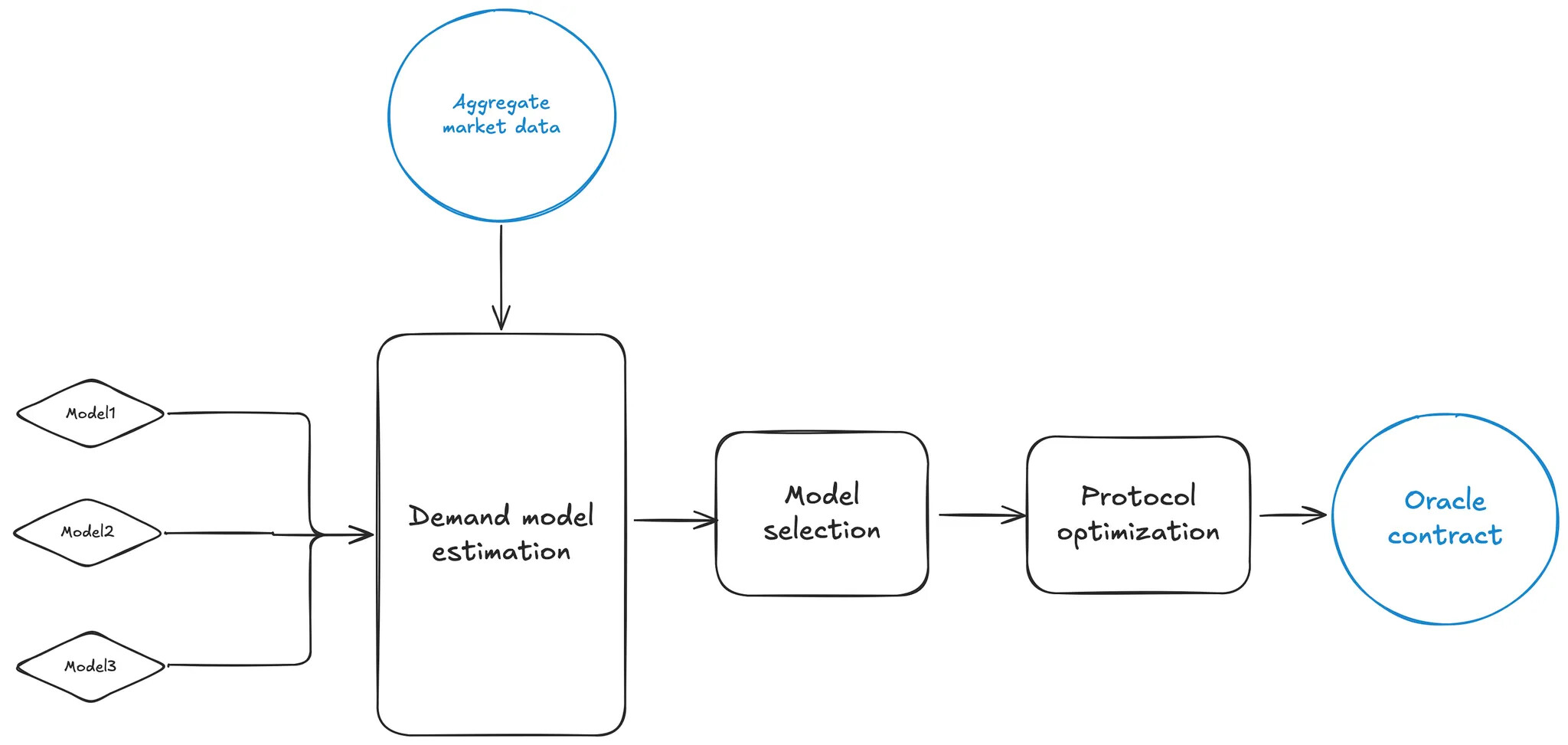
Chaos Labs proposes the implementation of a risk oracle to set optimal interest rate curves for stablecoins within the Aave protocol. We select a slope1 parameter that would lead to the best attainable protocol welfare, operationalized as constrained gross revenue, based on a dynamic analysis of borrowers’ aggregate responses to interest rate changes and total supply fluctuations. The primary components of the oracle architecture comprise:
Demand models - a demand model is an object that encapsulates certain assumptions about the behavior of protocol borrowers and specifies an approach to estimating the numeric parameters that pin down this behavior
Demand model estimation - given a demand model, parameters characterizing borrower behavior can be determined using aggregate market data, with the model’s accuracy evaluated out of sample
Model selection - the oracle pipeline estimates multiple demand models and evaluates their performance on out of sample historical data, so that the best model can be selected to drive the protocol optimization model
Protocol optimization - using the best demand model available to predict borrower response to interest rate changes, we determine the best slope parameter to maximize protocol welfare, subject to certain guardrails
The demand and protocol welfare models underlying the oracle transform aggregate market observables directly into a slope parameter recommendation, subject to programmable constraints implementing safety guardrails. As a concrete example, the constraints ensure that deviation from current parameter is appropriately restricted and that counterfactual demand induced by the optimal slope parameter does not breach utilization limits at any time.
Model flow
Motivation
Risk management requires setting parameters in a manner that safeguards the protocol against extreme events. Existing workflows that lead to particular recommendations for changes to protocol configuration, such as the shape of the interest rate curve, are driven by this consideration. We are proposing an oracle that would supplement this workflow, taking some of the critical elements of a risk configuration as a given and optimizing the protocol for an objective distinct from “minimizing bad debt accrual during periods of extreme volatility.” Here, we still treat risk management as the primary consideration, accepting some elements of the existing protocol configuration as an explicit constraint, while attempting to achieve constrained optimal protocol welfare.
The current approach for updating interest rates, utilizing the risk steward contract, allows for a maximum adjustment to the slope1 parameter of 100 bps every three days. However, this method requires considerable operational effort, as it involves manually creating a series of transactions to modify the interest rate curve across more than 60 stablecoin markets on 16 deployments, with a process akin to the one presented in Supply and Borrow Cap Risk Oracle Activation. This process becomes especially inefficient during repricing events, where the manual overhead and fundamental constraints hamper the ability to respond dynamically to changes in demand.
As Aave is the largest DeFi lending protocol, especially in terms of aggregate stablecoin liquidity, it effectively boasts the title of the primary market when deducing the market-priced interest rate on-chain. It is therefore essential to adopt a generalized, transparent, and robust methodology grounded in aggregate demand models—mathematically simple yet capable of generating meaningful predictions about future borrower behavior to optimize its configuration accordingly. By using multiple models and selecting the best ones dynamically, we ensure that the methodology is flexible enough to capture the evolving characteristics of demand for stablecoins, taking advantage of variation in supply to estimate demand model parameters. This approach does not rely on interest rate variation or any assumptions on the origin of existing interest rate curve parameters, making it robust to feedback loops.
Data
We model the demand, or total borrowing, as aggregate demand curves, or mathematical functions relating the prevailing market interest rate to demand. The particular shape of any such curve encodes the behavior of protocol borrowers in response to changes we make to the interest rate curve parameters. Each type of demand curve is defined by some parameters, which we can estimate using aggregate market data. The aggregate market data feeding into the model estimation component tracks total borrowing, supply and other market characteristics, such as the current interest rate curve settings, for supported chains, tokens and markets at a ~10-15 minute cadence. All estimation and protocol optimization utilize the observations at each update, although our analysis will use some quantities aggregated to daily or hourly levels, for the reader’s convenience.
Demand
Demand models
Conceptually, a demand model should be thought of as a triple consisting of a demand function, estimation objective and loss function. The demand function captures the aggregate change to total borrowing in response to a change in the interest rate curve. The estimation objective and loss function determine how the demand curve is fit to historical data.
The demand functions represent downward sloping aggregate demand, with some scale parameter A, characterizing the overall level of demand, and a parameter σ characterizing the elasticity, or the relative magnitude of the demand response to a change in interest rates.
Our demand functions are
isoelastic - Ax^σ, the elasticity parameter fixes the price elasticity at all points along the curve
exponential - Ae^(-σx)
linear - A + σx, the elasticity parameter is the slope of the line
Estimation objectives represent the deviation that the estimation program attempts to minimize according to some loss function
price - deviation from observed price, given the estimated demand and implied price
demand - deviation from observed demand
Finally, the loss functions are
L1 - minimizes the sum of absolute deviations, relatively insensitive to outliers
L2 - minimizes the sum of squared residuals
Consequently, we estimate a total of up to 12 different demand models for each run of the estimation and protocol welfare optimization pipeline, selecting the best one to serve as the representation of demand response for the protocol welfare optimization program.
Estimation
Model estimation strategy
In order to use a demand model for predicting counterfactual borrower response to adjustment in the interest rate curve parameters, we must recover the values of the scale and elasticity parameters from historical data. The demand model parameters for a particular function are estimated using non-linear regressions, minimizing the selected loss relative to the target determined by the objective. The particular choice of loss function determines the influence of outliers in the estimation. Minimizing loss can be thought of as finding a function in a particular class (e.g., isoelastic demand curves) that is “closest” to the observed data, with “closeness” measured by the chosen loss function. This “closest” function is identified, within its class, by the values of its parameters.
We do not compute standard errors or other explicitly statistical constructs, as we are concerned primarily with prediction rather than statistical inference. To elaborate on this further, the purpose of a typical econometric exercise of this nature, as might be performed by a practitioner of demand modeling in academia or economic consulting, is to determine the values of the demand function parameters in the service of making a point concerning a theoretical claim (e.g., that the demand should be either elastic, or inelastic). The predictions of a theoretical model of demand are assessed based on a fixed dataset, and subjected to a number of tests (e.g., for normality of the noise, model selection, etc.) to winnow the models down to a particular function, which is then usually estimated using a linear regression.
Our approach, while taking inspiration from standard economic models of demand, tackles the problem within a simple machine learning framework. We care most about the quality of our short-term predictions of demand response, rather than falsifying the predictions of some theoretical model. Consequently, we simply estimate the characteristics of demand on some window of data, and then predict its behavior on a disjoint time window of data to assess the quality of a particular model, that is, its out of sample fit.
In both the statistical and the machine learning approaches to modeling data-generating processes, overfitting is often a major concern. In the case of statistical models, overfitting results in poor estimation of model parameters and standard errors, while in the machine learning framework, it leads to poor out-of-sample fit. However, we restrict our models to fairly rigid functional forms, making overfitting essentially impossible.
The Appendix presents a detailed example of model definition and estimation for an isoelastic demand function with a price objective and an L2 loss function, with an explanation of how predictions are done on each prediction window.
Retrospective predictive fit
The estimating regressions are performed on a series of partially overlapping windows of data for each model, with predictions, used in model performance evaluation, made for some time frame following the estimation window. The predicted demand is then reconstructed for the entire period of interest to assess predictive fit. In the online estimation-prediction-optimization oracle workflow, we use the most recent window alone, but for subsequent analysis we will be using multiple windows.

Evaluation
The performance of different demand models within the prediction windows is assessed using a predictive fit measure, such as R^2, MASE (Mean Absolute Scaled Deviation) or a normalized sum of residuals. The latter measure most closely tracks “visual” fit, particularly in time-aggregated series, but is insensitive to variance. The best performing model is selected to serve as the basis for the protocol welfare optimization program.
Demand model selection
Any individual model cannot be relied upon to serve as the basis for protocol welfare optimization in all timeframes. This is because, ultimately, aggregate demand is an abstraction over individual behavior of many different participants in the protocol, each with unique risk preferences, token holdings and outside options for deployment of liquidity. Over time, all of these participant characteristics evolve. Additionally, some participants may enter and exit the protocol over time. This implies that having a fixed demand function representing aggregate demand across time is unlikely to correctly reflect the aggregate behavior of the participants. We operationalize the notion of “correctness” by retrospective predictive fit, that is, the degree to which out of sample prediction matches the actually observed behavior in the past.
Selecting a model on each of our moving prediction windows dynamically, we can significantly improve upon the performance of any given model. In fact, given the simplicity of our estimation approach, the predictive fit of the best-in-each-prediction-window model is surprisingly good. In the chart below, tracing demand and predicted demand from September 2024 to February 2025 for Aave’s Ethereum-core market, every window’s predicted demand is derived from the best-performing (according to the normalized sum of residuals measure) model for that window. Each window has an estimation timeframe of 7 days and a prediction timeframe of 3 days.

Protocol welfare model
Utilization-constrained protocol revenue as protocol welfare
There are several principles that guide our selection of aggregate protocol revenue as a measure of protocol welfare
- Every user with a healthy position is necessarily a supplier in an over-collateralized protocol
- Given the inherently risky nature of crypto markets, we can assume that the participants are, at least, risk-neutral
- User preference is always to make more money from the participation protocol for any fixed quantity of tokens supplied
Nevertheless, because crypto markets are punctuated by short periods of extreme volatility and severe price corrections, we have to explicitly guard against supply depletion to preclude even transient insolvencies from damaging public perceptions of the protocol’s security.
Following the principles and the considerations above, we define platform welfare as utilization-constrained aggregate supplier revenue. In formal terms, we will treat aggregate protocol revenue as the objective of an optimization program, while measures of maximal allowable utilization derived from analyses focused on extreme events are taken as a constraint on the counterfactual demand at the constrained optimal slope1.
Protocol optimization program
Effectively optimizing protocol welfare requires that the demand response to changes in the interest rate curve closely reflect the characteristics of underlying demand. Otherwise, the optimal interest rate curve parameter settings are optimal in name only, since the response of the borrowers to parameter changes cannot be effectively predicted.
We will assume that supply is a fixed quantity at every observation time. In principle, the supply side (which is, as we point out above, also the demand side) should be responsive to the prices we set. While it is possible, in principle, to formulate a more complex problem that considers both demand and supply response, we only consider the former, for tractability. Below, we present a minimal example of a protocol optimization program.
Let us introduce some symbolic quantities

We can now formulate a candidate optimization program for protocol welfare, normalizing both supply and demand by the total supply for illustration, so that we do not need to consider utilization separately from demand

The program aims to maximize revenue from interest accrual, subject to a realized utilization constraint, which requires that the demand response not result in utilization above some threshold for every single datapoint. This is an example of an essential guardrail, which ensures that the optimal solution respects a safeguard that we do not directly encode into the protocol objective.
Protocol optimization analysis
We perform the optimization of the slope1 parameter with responsive demand, using our prior demand model parameter estimates for this purpose, recomputing the counterfactual demand at each step in the optimization. To help us understand the operation and output of the protocol optimization model, we will examine the evolution of interest rate curves and the impact of relaxing the realized utilization constraint.
We illustrate the retrospective operation of our protocol optimization model using 2 months of data for USDC and USDT stablecoins within the Ethereum-core market for Aave V3. The timeframe ranges from 2024-12-24 to 2025-02-23. We let the slope parameter range over [0.01, 0.3], however, we impose a realized utilization constraint that guarantees that at no observation time does the counterfactual utilization demand at the optimum exceed a given threshold. As before, the estimation window size is 7 days and the prediction window size is 3 days. We restrict the model set to the 4 isoelastic demand function models for illustration, as other models can lead to greater variability in optimal slope values on this dataset.
Counterfactual Interest Rate Curve Parameters Evolution
The final output of a successful simulation model run is a new slope1 parameter, effectively defining a new interest rate curve as a function of utilization, which then evolves over time as the estimation and prediction windows move forward, as seen below for a realized utilization constraint of 91.5%, just slightly below the kink.
Over the timeframe under consideration, the total supply of both USDC and USDT is rising, but the demand is declining, leading to declining protocol revenues and low utilization.

The historical response to this was a gradual lowering of interest rates by decreasing the slope1 parameter, however, utilization continued to decline. Our protocol optimization model would have led to more aggressive downward adjustment.

Given our demand model estimates, this would have kept utilization close to the specified realized utilization constraint and much higher than what was achieved by the historical policy.

Higher utilization would have offset the lower interest rates, leading to greater revenue for the protocol.

Model operation and community feedback
Our approach relies on a necessarily reductive economic model of aggregate demand, which cannot incorporate all of the dynamic factors that influence real DeFi markets. The design, and specifically its underlying tooling, is a plug-and-play framework for benchmarking different protocol objectives, demand models and constraints, such as interest rate curve restrictions imposed by utilization incentive programs. This lets us leverage existing community expertise to iterate towards a better simulation model and maximal protocol welfare.
Triggers & limits
The proposed interest rate oracle leverages Edge Infrastructure to automate interest rate adjustments within set guardrails. Our methodology relies on accurate demand models to produce meaningful parameter recommendations. This means that indicators of demand behavior deviating from the last model used for protocol optimization should trigger a simulation run to refresh the demand models and produce a new parameter recommendation. A measure of deviation in observed demand can be given as

Additional triggers include breaches of specific guardrails, as well as time-triggers for regular updates.
- Excessive total borrowing deviation trigger
- Deviation from total borrowing implies that the underlying demand model requires a refresh
- Allows short-term average deviation to be greater than long-term average deviations, as the latter is a stronger indicator of the demand model going stale
- Short-term, 10 minutes to 1 hour (highest allowed aggregate deviation)
- Medium-term, 1 hour to 24 hours
- Long-term, 24 hours to 1 month (lowest allowed aggregate deviation)
- Utilization exceeding thresholds trigger
- Excessive utilization breaches a constraint we explicitly impose on the model
- Excessive utilization measures are operationalized as an aggregate function of time and distances from the threshold, evaluated over a defined interval
- Manual triggers
- Scheduled background back-testing and stress-testing simulations raise alerts to notify the risk management team of potentially advantageous updates even in the absence of significant deviations
- Observed utilization approaching the realized utilization threshold, an explicit model constraint, raises an alert to notify the risk management team of the need to review demand and interest rate behavior
The updates, similarly to those for the supply and borrow cap oracle, are limited in frequency and magnitude. Initially, frequency of regular updates and magnitude limits shall be set to 72 hours and 50 basis points respectively.
Appendix
Isoelastic demand with a price objective and an L2 loss function
Variables

Functional form
Assume that demand in each period has a constant price elasticity, or isoelastic, form

The elasticity parameter σ determines the % change in demand given a % change in price, at all prices along the curve. The scaling parameter A is the level of fully inelastic demand. The observable quantities, supply and demand, are interpreted to be USD. Price is assumed to be periodic interest rate as a decimal. Note that the choice of price scaling (e.g., periodic rate, APR, or $ cost to borrow a $1) is consequential to elasticity estimates, unless it is multiplicative.
Given the assumption of constant price elasticity for the demand, it follows that, in each period, demand, supply and price must satisfy the following equation

The price mapping is assumed to be continuous and monotonically increasing in utilization ut = Dt / St, though in the particular markets belonging to the Aave platform that we will be dealing with, they take a specific piece-wise linear form

Estimation of demand parameters
We take a simple machine learning style approach to determining the demand function parameters, numerically solving the following optimization program

The solution minimizes the Euclidean distance between demand implied by the constant elasticity form and observed demand vectors, or the “sum of squared residuals,” as it is usually known in econometrics.
Alternatively, the optimization program could be reformulated to minimize distance to the observed price vector

These optimization programs should be equivalent under our assumptions. That is, if we were to observe some data generating process arising from random variation of a flat supply curve, generating the observables (D, P)t, the solutions to the programs would be the same. However, in practice we do not observe such a process. We also encounter issues with numerical optimization algorithms, making the choice of a particular formulation consequential and encouraging the use of multiple models in practice.
Prediction of future demand
Because of the mechanical linkage between utilization and interest rate, observed demand and prices are positively correlated. However, we are estimating the parameters of a demand curve that is expected to be downward sloping (i.e., “holding everything else equal,” demand should decrease as prices increase).
Taking into account the linkage through the interest rate curve, in each time period we can predict future demand by numerically solving the following equation
